Searching for ArcticDEM and REMA strips

This notebook is available on GitHub here.

Here, we describe how we can use pdemtools to search for, and download, ArcticDEM and REMA strips.

First, we must import pdemtools, in addition to the in-built os function for file management and matplotlib to plot our results in this notebook.

import os

import pdemtools as pdt
import matplotlib.pyplot as plt

plt.rcParams['figure.constrained_layout.use'] = True
plt.rcParams['font.sans-serif'] = "Arial"

%matplotlib inline

Searching for strips

For the example here, let’s examine recent surface elevation change across KIV Steenstrups Nordre Bræ (where we know significant change occurred between 2016 and 2021).

We can query all available ArcticDEM or REMA by using the pdt.search() function. By default, the search function automatically connects to the PGC STAC API, and the function essentially wraps a pystac_client query with a few additional bells and whistles, such as being able to query by the fractional coverage of your AOI. If you don’t know what STAC or pystac_client is, that’s fine - this tool is designed to help you engage with ArcticDEM/REMA data without getting into the weeds!

If for whatever reason, you would rather query a local source (e.g. you anticipate not having access to the internet), you can instead provide the local PGC index file location to the optional index_fpath parameter. For more information on this, see the ‘Supplementary datasets’ page.

To use the pdt.search() function, set an appropriate bounding box ([xmin, ymin, xmax, ymax]in EPSG:3413 / Polar Stereographic North*), and set further filtering choices to limit our options to high-quality, summer scenes that cover at least 70% of the bounding box.

⚠️ NOTE: pDEMtools currently only accepts bounds in the same format as the ArcticDEM/REMA datasets themselves: that is say, the Polar Stereographic projections (EPSG:3413 for the north/ArcticDEM and EPSG:3031 for the south/REMA).

bounds = (459000, -2539000, 473000, -2528000)

gdf = pdt.search(
    dataset='arcticdem',
    bounds = bounds,
    dates = '20170101/20221231',
    months = [6,7,8,9],
    years = [2017,2021],
    baseline_max_hours = 24,
    sensors=['WV03', 'WV02', 'WV01'],
    accuracy=2,
    min_aoi_frac = 0.7,
)

print(f'{len(gdf)} strips found')

6 strips found

⚠️ NOTE: Including both dates and years as parameters in this use case is strictly redundant (because e.g. dates = '20190101/20191231' is functionally identical to years = 2019). However, it is worth highlighting that both options are avaiable to you!

The pdt.search() function returns a geopandas geodataframe, which we can visualise as with any other dataframe. There are many columns containing a variety of different data. These columns will differ depending on whether you sourced the data from the online STAC (default) or a local index file - as result, pdemtools appends the most useful data as columns beginning with pdt_*: ['pdt_id', 'pdt_datetime1', 'pdt_datetime2', 'pdt_dem_baseline_hours', 'pdt_datetime_mean', 'pdt_year', 'pdt_month', 'pdt_aoi_frac']. Here, let’s take a look at the strip IDs and the acquisition dates of the two WorldView scenes that went into making the DEM:

gdf[['pdt_id', 'pdt_datetime1', 'pdt_datetime2']]

	pdt_id	pdt_datetime1	pdt_datetime2
0	SETSM_s2s041_WV01_20170607_1020010063D4CE00_10...	2017-06-07 16:36:42+00:00	2017-06-07 16:37:31+00:00
1	SETSM_s2s041_WV01_20170624_1020010060B7D000_10...	2017-06-24 16:35:53+00:00	2017-06-24 16:36:43+00:00
2	SETSM_s2s041_WV03_20170728_104001002E870C00_10...	2017-07-28 14:05:24+00:00	2017-07-28 14:06:24+00:00
3	SETSM_s2s041_WV02_20170829_103001006F1D6400_10...	2017-08-29 14:21:43+00:00	2017-08-29 14:23:03+00:00
4	SETSM_s2s041_WV03_20210715_104001006A09A000_10...	2021-07-15 13:55:42+00:00	2021-07-15 13:56:37+00:00
5	SETSM_s2s041_WV02_20210731_10300100C359CF00_10...	2021-07-31 14:09:25+00:00	2021-07-31 14:10:48+00:00

There’s still no guarantee that these scenes will be of high quality - so we can make use of the load.preview() function to download a 10 m hillshade that will help us quickly asses strip quality. Note that we can rerun this cell repeatedly, changing the value of i to a different index number to previous different scenes.

# =================
# SCENE TO PREVIEW
i = 5
# =================

preview = pdt.load.preview(gdf.iloc[[i]], bounds)

fig, ax = plt.subplots(layout='constrained')
preview.plot.imshow(cmap='Greys_r', add_colorbar=False)

gdf.iloc[[i]].plot(ax=ax, fc='none', ec='tab:red')

ax.set_title(gdf.iloc[[i]].pdt_datetime1.dt.date.values[0])
plt.show()

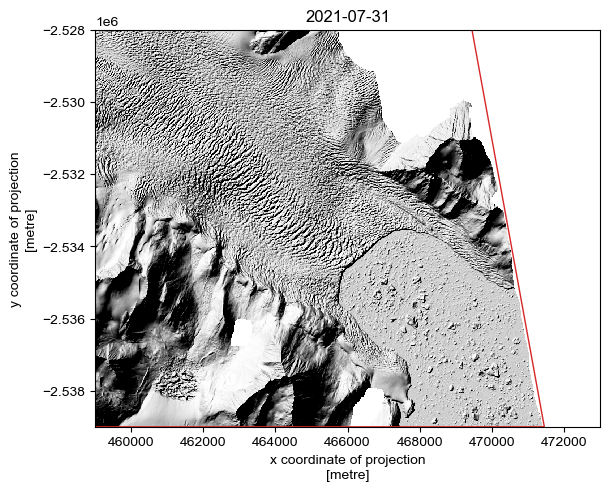
By examining the individual strips one-by-one, we can manually identify the optimal scenes for our purpose.

⚠️ NOTE: The preview() option draws on PGC-provided data, which is automatically masked according to the PGC bitmask. It is entirely possible that the search() function can return a valid datastrip that covers a sufficient proportion of the AOI to meet the min_aoi_frac requirements, but it will appear empty (i.e. all-NaN) when viewed. The preview() function will help you identify these ‘empty’ scenes, but there may still be (poor-quality) data present if it is downloaded using the load.from_search() function with bitmask=False. However, by default, load.from_search()defaults to bitmask = True.

Here, I have selected the second and sixth strips (index positions 1 and 5)

selected_scenes = [1, 5]

Let’s save the selected scenes as a geopackage, so we can return to this later:

if not os.path.exists('example_data'):
    os.mkdir('example_data')

gdf_sel = gdf.iloc[selected_scenes]

gdf_sel.to_file(os.path.join('example_data', 'scenes.gpkg'))

gdf_sel

	geometry	gsd	title	created	license	rmse	proj:code	published	is_lsf	proj:shape	...	href_hillshade	href_hillshade_masked	pdt_id	pdt_datetime1	pdt_datetime2	pdt_dem_baseline_hours	pdt_datetime_mean	pdt_year	pdt_month	pdt_aoi_frac
1	POLYGON Z ((459000 -2539000 0, 459000 -2528000...	2.0	SETSM_s2s041_WV01_20170624_1020010060B7D000_10...	2021-11-07T04:24:10Z	CC-BY-4.0	-9999	EPSG:3413	2022-09-22T05:38:17Z	True	[11287, 12320]	...	https://pgc-opendata-dems.s3.us-west-2.amazona...	https://pgc-opendata-dems.s3.us-west-2.amazona...	SETSM_s2s041_WV01_20170624_1020010060B7D000_10...	2017-06-24 16:35:53+00:00	2017-06-24 16:36:43+00:00	0.0	2017-06-24 16:36:18+00:00	2017	6	1.000000
5	POLYGON Z ((471450.48 -2539000 0, 459000 -2539...	2.0	SETSM_s2s041_WV02_20210731_10300100C359CF00_10...	2021-11-07T04:32:49Z	CC-BY-4.0	-9999	EPSG:3413	2022-09-22T05:38:21Z	True	[48497, 17156]	...	https://pgc-opendata-dems.s3.us-west-2.amazona...	https://pgc-opendata-dems.s3.us-west-2.amazona...	SETSM_s2s041_WV02_20210731_10300100C359CF00_10...	2021-07-31 14:09:25+00:00	2021-07-31 14:10:48+00:00	0.0	2021-07-31 14:10:06.500000+00:00	2021	7	0.817726

2 rows × 51 columns

Downloading the strips

From the geopandas dataframe, we can extract key information such as the DEM ID and dates:

date_1 = gdf_sel.iloc[[0]].pdt_datetime1.dt.date.values[0]
dem_id_1 = gdf_sel.iloc[[0]].pdt_id.values[0]

date_2 = gdf_sel.iloc[[1]].pdt_datetime2.dt.date.values[0]
dem_id_2 = gdf_sel.iloc[[1]].pdt_id.values[0]

But we needn’t do all this just to downlad a strip, as the load.from_search() function will accept a dataframe row directly. Let’s make a little function to download and save the data - we can save the dem using the rioxarray accessor function .rio.to_raster().

def download_scene(gdf_row, dem_id, bounds=bounds, output_directory='example_data'):

    out_fpath = os.path.join(output_directory, f'{dem_id}.tif')

    if not os.path.exists(out_fpath):

        dem = pdt.load.from_search(gdf_row, bounds=bounds, bitmask=True)

        dem.rio.to_raster(out_fpath, compress='ZSTD', predictor=3, zlevel=1)

        return dem

    else:

        return pdt.load.from_fpath(out_fpath, bounds=bounds)

Note, these are 2 m strips that will take a while to download! To save on added time when rerunning this notebook, I’ve added an additional test to the function: if we’ve already downloaded the DEM and saved it to the local directory, this function will instead load it from the local file location using the load.from_fpath() function.

⚠️ NOTE: More advanced geospatial python users may wish to note that DEMs can be loaded as dask arrays, enabling lazy evaluation and only triggering download when required by a further command. This is done providing a chunks parameter to load.from_search(), load.from_id(), or load.mosaic() (e.g.(50, 50), True, "auto"), as is the case for the ``rioxarray.load_rasterio()` function that it wraps <https://corteva.github.io/rioxarray/html/rioxarray.html#rioxarray-open-rasterio>`__.

Regardless, we can now use this function to select and download relevant rows from our geodataframe using the standard Pandax indexing method (DataFrame.iloc[[i]], where i is the desired row index):

dem_1 = download_scene(gdf_sel.iloc[[0]], dem_id_1, bounds)

dem_2 = download_scene(gdf_sel.iloc[[1]], dem_id_2, bounds)

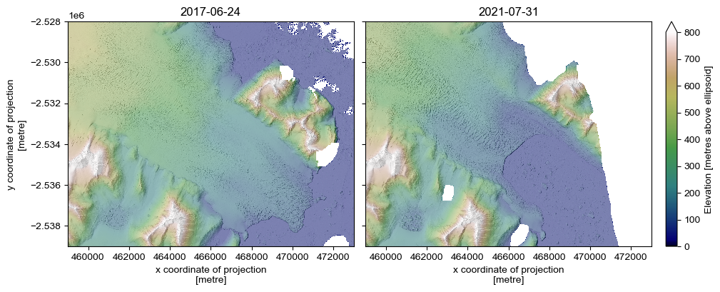
Let’s plot up one of the DEMs, taking advantage of the in-built hillshade generation function:

hillshade_1 = dem_1.pdt.terrain('hillshade', hillshade_multidirectional=True, hillshade_z_factor=2)
hillshade_2 = dem_2.pdt.terrain('hillshade', hillshade_multidirectional=True, hillshade_z_factor=2)

fig, axes = plt.subplots(layout='constrained', ncols=2, figsize=(10,3.9), sharex=True, sharey=True)

ax = axes[0]
dem_1.plot.imshow(cmap='gist_earth', vmin=0, vmax=800, ax=ax, add_colorbar=False) # cbar_kwargs={'label': 'Elevation [metres above ellipsoid]'})
hillshade_1.plot.imshow(cmap='Greys_r', alpha=.5, ax=ax, add_colorbar=False)
ax.set_aspect('equal')
ax.set_title(date_1)

ax = axes[1]
dem_2.plot.imshow(cmap='gist_earth', vmin=0, vmax=800, ax=ax, cbar_kwargs={'label': 'Elevation [metres above ellipsoid]'})
hillshade_2.plot.imshow(cmap='Greys_r', alpha=.5, ax=ax, add_colorbar=False)
ax.set_ylabel(None)
ax.set_aspect('equal')
ax.set_title(date_2)

plt.show()

Change through time

As the surface height changes between these two images is particularly large (on the order of 100 m), we can get a first-order approximation of surface change by subtracting the latter image from the first:

dz = (dem_2 - dem_1)

fig, ax = plt.subplots(layout='constrained', figsize=(7,4.7))

vrange = 200
dz.plot.imshow(cmap='coolwarm', vmin=-vrange, vmax=vrange, cbar_kwargs={'label': 'ΔZ [m]'})
hillshade_1.plot.imshow(cmap='Greys_r', alpha=.5, add_colorbar=False)

ax.set_aspect('equal')
ax.set_title(f'{date_2} - {date_1}')

plt.show()

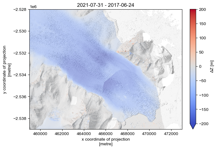
You might notice some odd patches of colour in the off-ice region. This is because rigorous DEM differencing necessitates coregistering scenes. pDEMtools provides functions to faciliate a common iterative method of coregistration, which we explore in the ‘Coregistration’ tutorial.