Downloading ArcticDEM and REMA mosaics

This notebook is available on GitHub here.

pdemtools provides a simple way to download ArcticDEM and REMA mosaics, as well as derive simple geomorphometry such as hillshades, slopes, and curvatures.

First, we must import pdemtools, in addition to the in-built os library for file management and matplotlib to plot our results in this notebook.

import os

import pdemtools as pdt
import matplotlib.pyplot as plt

plt.rcParams['figure.constrained_layout.use'] = True
plt.rcParams['font.sans-serif'] = "Arial"

%matplotlib inline

Load mosiac

To load mosaics from the PGC AWS bucket, we can make use of the pDEMtools’ load.mosaic() function.

All we need is the bounds of our area of interest. This can be a tuple (in the format (xmin, ymin, xmax, ymax)) or a shapely geometry. Note that pDEMtools currently only accepts bounds in the same format as the ArcticDEM/REMA datasets themselves: that is say, the Polar Stereographic projections (EPSG:3413 for the north/ArcticDEM and EPSG:3031 for the south/REMA).

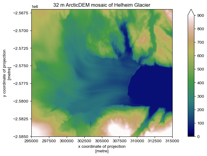
For this example, let’s set the bounds to take a look at Helheim Glacier:

bounds = (295000, -2585000, 315000, -2567000)

Now we can use the pdemtools.mosaic() function, specificying the dataset ('arcicdem' or 'rema'), resolution (which can be either 2, 10, or 32 metres), and the aforementioned bounding box. Note that, at this step, we are downloading the data from the AWS bucket, so 2 m resolution mosaics may take a while to download. Let’s download the 32 m mosaic for now:

%%time
dem = pdt.load.mosaic(
    dataset='arcticdem',  # must be `arcticdem` or `rema`
    resolution=32,        # must be 2, 10, or 32
    bounds=bounds,        # (xmin, ymin, xmax, ymax) or a shapely geometry
    version='v4.1',       # optional: desired version (defaults to most recent)
)

CPU times: user 228 ms, sys: 79.3 ms, total: 307 ms
Wall time: 6.8 s

pDEMtool functions return rioxarray-compatible xarray DataArrays (see here for an introduction), meaning you can take advantage of all relevant functionality, such as saving:

if not os.path.exists('example_data'):
    os.mkdir('example_data')

dem.rio.to_raster(os.path.join('example_data', 'helheim_arcticdem_mosaic_32m.tif'), compress='ZSTD', predictor=3, zlevel=1)

Or plotting:

fig, ax = plt.subplots(figsize=(7, 5))

dem.plot.imshow(ax=ax, cmap='gist_earth', vmin=0, vmax=900)

ax.set_aspect('equal')
ax.set_title('32 m ArcticDEM mosaic of Helheim Glacier')
plt.show()

Postprocessing

pDEMtools introduces a handy xarray accessor for performing preliminary preprocessing and assessment. These aren’t intended to be as full-featured as some other excellent community tools, such as xdem or richdem, but it is hoped that they are specific to the sort of uses that ArcticDEM and REMA users might want (e.g. a focus on ice sheet and cryosphere work), as well as the particular strengths of ArcticDEM and REMA datasets (high-resolution and multitemporal).

Geoid Correction

By taking advantage of a local copy of the Greenland or Antarctica BedMachine, the data module’s geoid_from_bedmachine() function can be used to quickly extract a valid EIGEN-6C4 geoid, reprojected and resampled to match the study area. First, let’s specify the location of BedMachine on our local system:

bedmachine_fpath = '.../BedMachineGreenland-v5.nc'

geoid = pdt.data.geoid_from_bedmachine(bedmachine_fpath, dem)

If you wish to use a different geoid (for instance, you are interested in a region outside of Greenland or Antarctica) you can also use your own geoid, loaded via xarray. To aid with this, a geoid_from_raster() function is also included in the data module, accepting a filepath to a rioxarray.open_rasterio()-compatible file type.

After getting our geoid, we can correct the DEM by feeding the geoid to the .pdt.geoid_correct() function.

dem_geoidcor = dem.pdt.geoid_correct(geoid)

Sea Level Filtering

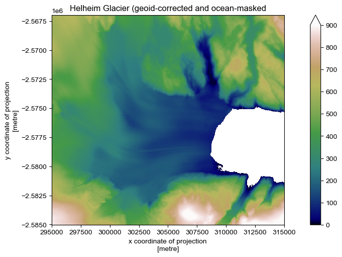
We can also filter out sea level from geoid-corrected DEMs, adapting the method of Shiggins et al. (2023) to detect sea level.

In this workflow, sea-level is defined as the modal 0.25 m histogram bin between +10 and -10 metres above the geoid. If there is not at least 1 km2 of surface between these values, then the DEM is considered to have no signficant ocean surface. DEM surface is masked as ocean where the surface is within 5 m of the detected sea level.

All of these values can be modified as input variables, but to stick with the defaults we can leave as-is:

dem_masked = dem_geoidcor.pdt.mask_ocean(near_sealevel_thresh_m=5)

fig, ax = plt.subplots(figsize=(7, 5))

dem_masked.plot.imshow(ax=ax, cmap='gist_earth', vmin=0, vmax=900)

ax.set_aspect('equal')
ax.set_title('Helheim Glacier (geoid-corrected and ocean-masked')
plt.show()

Although it is not the case for the new (v.4.1) ArcticDEM mosaic, when examining individual strips or older mosaics, icebergs will remain unmasked. This is reflective of the original purpose of the Shiggins et al. (2023) method, which was to identify icebergs!

If desired, we can resolve this by filtering out smaller groups of pixels. pDEMtools offers this function as part of the .pdt.mask_icebergs() function, which wraps the cv2.connectedComponentsWithStats function to filter out contiguous areas beneath a provided area threshold (defaults to 1e6 m2, i.e. 1 km2)

dem_masked = dem_masked.pdt.mask_icebergs(area_thresh_m2=1e6)

The geoid correction and sea level filtering routines are useful for both mosaic and strip presentation and analysis!