Strip search and coregistraion#

This notebook is available on GitHub here.

Here, we describe how we can use pdemtools to search for, and download, ArcticDEM and REMA strips. We also coregister them, allowing for simple change analysis to be performed.

First, we must import pdemtools, in addition to the in-built os function for file management and matplotlib to plot our results in this notebook.

[1]:

import os

import pdemtools as pdt

import matplotlib.pyplot as plt

plt.rcParams['figure.constrained_layout.use'] = True
plt.rcParams['font.sans-serif'] = "Arial"

%matplotlib inline

We will also need to provide the local location of the ArcticDEM strip index and ArcticDEM bedmachine product. These do not need to be in any specific directory - just provide the complete filepath as a string.

[2]:

index_fpath = '.../ArcticDEM_Strip_Index_s2s041.parquet'
bm_fpath = '.../BedMachineGreenland-v5.nc'

Searching for strips#

For the example here, let’s example recent surface elevation change across KIV Steenstrups Nordre Bræ (where we know significant change occurred between 2016 and 2021).

Let’s set an appropriate bounding box (in EPSG:3413 / Polar Stereographic North*), and set further filtering choices to limit our options to high-quality, summer scenes that cover at least 70% of the bounding box.

*Note that pDEMtools currently only accepts bounds in the same format as the ArcticDEM/REMA datasets themselves: that is say, the Polar Stereographic projections (EPSG:3413 for the north/ArcticDEM and EPSG:3031 for the south/REMA).

[3]:

bounds = (459000, -2539000, 473000, -2528000)

gdf = pdt.search(
    index_fpath,
    bounds,
    dates = '20170101/20221231',
    months = [6,7,8,9],
    years = [2017,2021],
    baseline_max_hours = 24,
    sensors=['WV03', 'WV02', 'WV01'],
    accuracy=2,
    min_aoi_frac = 0.7,
)

gdf = gdf.sort_values('acqdate1')

print(f'{len(gdf)} strips found')

6 strips found

Note that including both dates and years as parameters in this use case is strictly redundant (because e.g. dates = '20190101/20191231' is functionally identical to years = 2019). However, it is worth highlighting that both options are avaiable to you! .

The pdt.search() function returns a geopandas geodataframe, which we can visualise as with any other dataframe:

[4]:

gdf[['dem_id', 'acqdate1', 'acqdate2']]

[4]:

	dem_id	acqdate1	acqdate2
175143	SETSM_s2s041_WV01_20170607_1020010063D4CE00_10...	2017-06-07 16:36:42+00:00	2017-06-07 16:37:31+00:00
175148	SETSM_s2s041_WV01_20170624_1020010060B7D000_10...	2017-06-24 16:35:53+00:00	2017-06-24 16:36:43+00:00
175138	SETSM_s2s041_WV03_20170728_104001002E870C00_10...	2017-07-28 14:06:24+00:00	2017-07-28 14:05:24+00:00
175116	SETSM_s2s041_WV02_20170829_103001006F1D6400_10...	2017-08-29 14:23:03+00:00	2017-08-29 14:21:43+00:00
175106	SETSM_s2s041_WV03_20210715_104001006A09A000_10...	2021-07-15 13:56:37+00:00	2021-07-15 13:55:42+00:00
175144	SETSM_s2s041_WV02_20210731_10300100C359CF00_10...	2021-07-31 14:10:48+00:00	2021-07-31 14:09:25+00:00

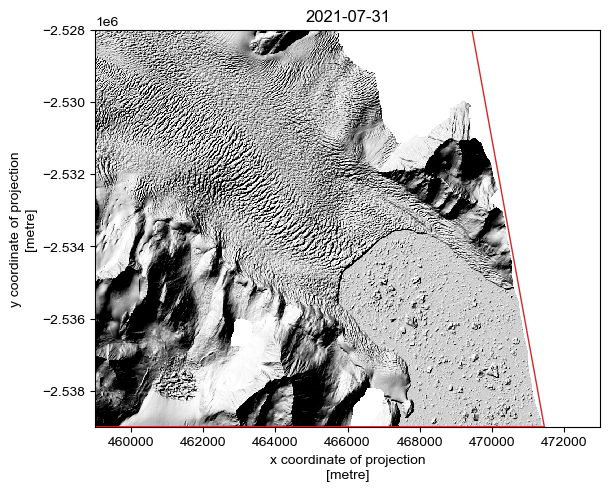
There’s still no guarantee that these scenes will be of high quality - so we can make use of the load.preview() function to download a 10 m hillshade that will help us quickly asses strip quality. Note that we can rerun this cell repeatedly, changing the value of i to a different index number to previous different scenes.

[5]:

# =================
# SCENE TO PREVIEW
i = 5
# =================

preview = pdt.load.preview(gdf.iloc[[i]], bounds)

fig, ax = plt.subplots(layout='constrained')
preview.plot(cmap='Greys_r', add_colorbar=False)

gdf.iloc[[i]].plot(ax=ax, fc='none', ec='tab:red')

ax.set_title(gdf.iloc[[i]].acqdate1.dt.date.values[0])
plt.show()

../_images/examples_strip_search_and_dem_difference_11_0.png

By examining the individual strips one-by-one, we can manually identify the optimal scenes for our purpose.

NOTE: The preview() option draws on PGC-provided data, which is automatically masked according to the PGC bitmask. It is entirely possible that the search() function can return a valid datastrip that covers a sufficient proportion of the AOI to meet the min_aoi_frac requirements, but it will appear empty (i.e. all-NaN) when viewed. The preview() function will help you identify these ‘empty’ scenes, but there may still be (poor-quality) data present if it is downloaded using the load.from_search() function with bitmask=False. However, by default, load.from_search()defaults to bitmask = False.

Here, I have selected the second and sixth strips (index positions 1 and 5)

[6]:

selected_scenes = [1, 5]

Let’s save the selected scenes as a geopackage, so we can return to this later:

[7]:

if not os.path.exists('example_data'):
    os.mkdir('example_data')

[8]:

gdf_sel = gdf.iloc[selected_scenes]

gdf_sel.to_file(os.path.join('example_data', 'scenes.gpkg'))

gdf_sel

[8]:

	fid	dem_id	pairname	stripdemid	sensor1	sensor2	catalogid1	catalogid2	acqdate1	acqdate2	...	fileurl	s3url	geom	pdt_time1	pdt_time2	pdt_dem_baseline_hours	pdt_time_mean	pdt_year	pdt_month	pdt_aoi_frac
175148	175149	SETSM_s2s041_WV01_20170624_1020010060B7D000_10...	WV01_20170624_1020010060B7D000_1020010063B5E200	WV01_20170624_1020010060B7D000_1020010063B5E20...	WV01	WV01	1020010060B7D000	1020010063B5E200	2017-06-24 16:35:53+00:00	2017-06-24 16:36:43+00:00	...	https://data.pgc.umn.edu/elev/dem/setsm/Arctic...	https://polargeospatialcenter.github.io/stac-b...	POLYGON ((459000 -2539000, 459000 -2528000, 47...	2017-06-24 16:35:53+00:00	2017-06-24 16:36:43+00:00	0.0	2017-06-24 16:36:18+00:00	2017	6	1.000000
175144	175145	SETSM_s2s041_WV02_20210731_10300100C359CF00_10...	WV02_20210731_10300100C359CF00_10300100C37C8000	WV02_20210731_10300100C359CF00_10300100C37C800...	WV02	WV02	10300100C359CF00	10300100C37C8000	2021-07-31 14:10:48+00:00	2021-07-31 14:09:25+00:00	...	https://data.pgc.umn.edu/elev/dem/setsm/Arctic...	https://polargeospatialcenter.github.io/stac-b...	POLYGON ((471450.48 -2539000, 459000 -2539000,...	2021-07-31 14:10:48+00:00	2021-07-31 14:09:25+00:00	1.0	2021-07-31 14:10:06.500000+00:00	2021	7	0.817726

2 rows × 40 columns

Downloading the strips#

From the geopandas dataframe, we can extract key information such as the DEM ID and dates:

[9]:

date_1 = gdf_sel.iloc[[0]].acqdate1.dt.date.values[0]
dem_id_1 = gdf_sel.iloc[[0]].dem_id.values[0]

date_2 = gdf_sel.iloc[[1]].acqdate1.dt.date.values[0]
dem_id_2 = gdf_sel.iloc[[1]].dem_id.values[0]

But we needn’t do all this just to downlad a strip, as the load.from_search() function will accept a dataframe row directly. Let’s make a little function to download and save the data - we can save the dem using the rioxarray accessor function .rio.to_raster():

[10]:

def download_scene(gdf_row, dem_id, output_directory='example_data'):

    dem = pdt.load.from_search(gdf_row, bounds=bounds, bitmask=True)

    dem.compute()  # rioxarray uses lazy evaluation, so we can force the download using the `.compute()` function.

    dem.rio.to_raster(os.path.join(output_directory, f'{dem_id}.tif'), compress='ZSTD', predictor=3, zlevel=1)

    return dem

And now, we can select relevant rows from our geodataframe using the standard Pandax indexing method (DataFrame.iloc[[i]], where i is the desired row index)

[11]:


dem_1 = download_scene(gdf_sel.iloc[[0]], dem_id_1)

[12]:


dem_2 = download_scene(gdf_sel.iloc[[1]], dem_id_2)

These are 2 m strips that will take a while to download! However, if you have saved them locally, as we have above, getting them back into the script without downloading is as simple as using the load.from_fpath() function:

[13]:

dem_1 = pdt.load.from_fpath(os.path.join('example_data', f'{dem_id_1}.tif'), bounds=bounds)

[14]:

dem_2 = pdt.load.from_fpath(os.path.join('example_data', f'{dem_id_2}.tif'), bounds=bounds)

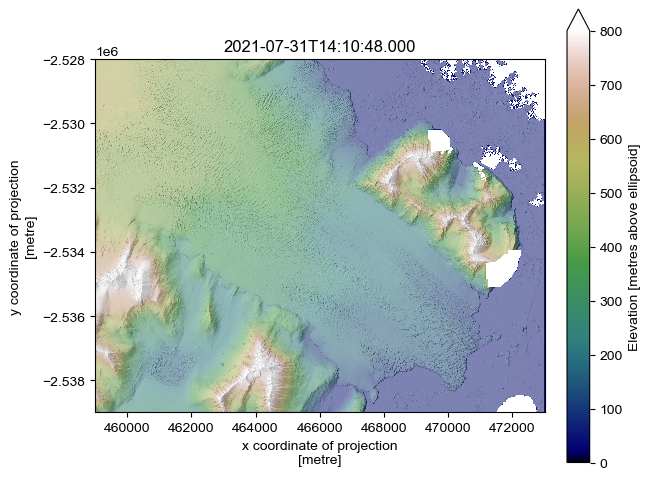
Let’s plot up one of the DEMs, taking advantage of the in-built hillshade generation function:

[15]:

hillshade_1 = dem_1.pdt.terrain('hillshade', hillshade_multidirectional=True, hillshade_z_factor=2)

[16]:

fig, ax = plt.subplots(layout='constrained')

dem_1.plot(cmap='gist_earth', vmin=0, vmax=800, cbar_kwargs={'label': 'Elevation [metres above ellipsoid]'})

hillshade_1.plot(cmap='Greys_r', alpha=.5, add_colorbar=False)

ax.set_aspect('equal')
ax.set_title(gdf.iloc[[i]].acqdate1.values[0])
plt.show()

../_images/examples_strip_search_and_dem_difference_30_0.png

Coregistration and DEM differencing#

Rigorous DEM differencing necessitates coregistering scenes. pDEMtools includes a couple functions to make this quick and easy. Only provides one method of coregistration is provided, that of Nuth and Kääb (2011), which accounts for translation errors only. For further options (e.g. rotation correction), it is worth consulting the xdem package.

First, we must set a region of stable ground to coregister too. Around Antarctica and Greenland, we can base this on the mask included within BedMachine. The data.bedrock_mask_from_bedmachine() function makes this easy:

[17]:

bedrock_mask = pdt.data.bedrock_mask_from_bedmachine(bm_fpath, dem_1)

Then we can coregister dem_2 against dem_1 using the .pdt.coregister() function. This is based on code used in the PGC postprocessing pipeline, updated to utilise the updated pdemtools geomorphometric variable derivation.

[18]:

dem_2_coreg = dem_2.pdt.coregister(dem_1, bedrock_mask)

Planimetric Correction Iteration 1
Offset (z,x,y): 0.000, 0.000, 0.000
RMSE = 5.008943557739258
Planimetric Correction Iteration 2
Offset (z,x,y): -0.506, -5.149, 5.180
Translating: -0.51 Z, -5.15 X, 5.18 Y

/Users/tom/miniforge3/envs/geospatial/lib/python3.12/site-packages/osgeo/gdal.py:312: FutureWarning: Neither gdal.UseExceptions() nor gdal.DontUseExceptions() has been explicitly called. In GDAL 4.0, exceptions will be enabled by default.
  warnings.warn(

RMSE = 3.56615948677063
Planimetric Correction Iteration 3
Offset (z,x,y): -0.281, -5.238, 5.126
Translating: -0.28 Z, -5.24 X, 5.13 Y
RMSE = 3.5588386058807373
Planimetric Correction Iteration 4
Offset (z,x,y): -0.276, -5.241, 5.124
Translating: -0.28 Z, -5.24 X, 5.12 Y
RMSE = 3.5588457584381104
RMSE step in this iteration (0.00001) is above threshold (-0.001), stopping and returning values of prior iteration.
Final offset (z,x,y): -0.281, -5.238, 5.126
Final RMSE = 3.5588386058807373

Sometimes, if one of the DEMs is smaller than the clip region, this can fail. If this is the case, try ‘padding’ the DEMs with NaN values to the full AOI, e.g.:

dem = dem.rio.pad_box(*bounds, constant_values=np.nan)

Let’s compare and plot:

[19]:

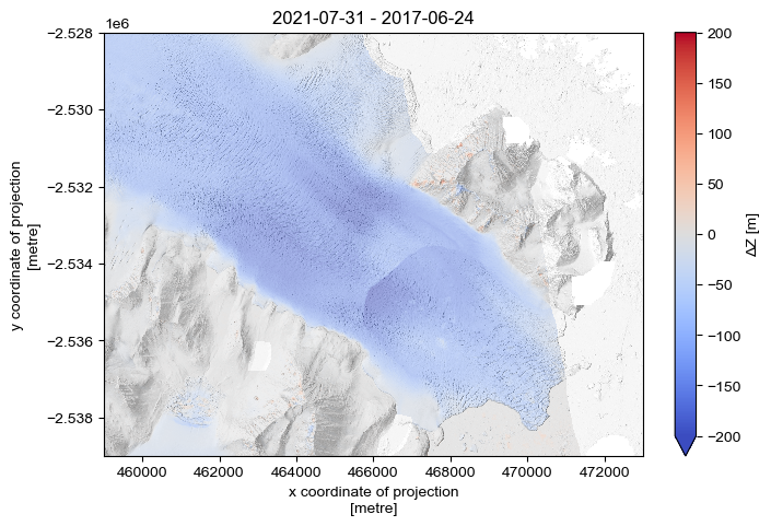
dz_coreg = (dem_2_coreg - dem_1)

[20]:

fig, ax = plt.subplots(layout='constrained', figsize=(7,4.7))

vrange = 200
dz_coreg.plot(cmap='coolwarm', vmin=-vrange, vmax=vrange, cbar_kwargs={'label': 'ΔZ [m]'})
hillshade_1.plot(cmap='Greys_r', alpha=.5, add_colorbar=False)

ax.set_aspect('equal')
ax.set_title(f'{gdf_sel.iloc[[1]].acqdate1.dt.date.values[0]} - {gdf_sel.iloc[[0]].acqdate1.dt.date.values[0]}')

plt.savefig(os.path.join('..', 'images', 'example_dem_difference.jpg'), dpi=300)
plt.show()

Strip search and coregistraion

Contents

Strip search and coregistraion#

Searching for strips#

Downloading the strips#

Coregistration and DEM differencing#